Game Theory and Decision Theory

Statistics starts with probability theory, particularly in the analysis of games of chance. To be refferred to as a game, it involves three elements mathmatically:

1. Parameter space \(\Theta\), a population characteristics, a physical quantity for example, mean.

2. Actions/Decisions space \(\mathscr{D}\) available to statistician.

3. A loss function, \(L(\theta,d)\), a real-valued function defined on \(\Theta \times \mathscr{D}\).

Thus, any such triplet \((\Theta, \mathscr{D}, L )\) defines a game. For example, Black jack, poker, chess, tic-tac-toe and so on are games that are played by strategy. “Game Theory” was proposed by two economists: John Von Neuman and John Nash in 1950s. Two or more players competing against one another. Neither player generally knows the others’ strategy. The goal of the game is to pick a strategy that guarentees he/she can’t be “too bad”.

Real life examples:

Product pricing decisions: Seasonal promotions allow retailers to sell more stock of products and consumers to get best deals. The focus of retailers is on using the best pricing strategy while the preference of consumers is to choose the best deal in terms of discount and variety.

Investment decisions: The different distributions of the investment on bond, stocks, short-term reserves will result in different returns. A historical risk/return (1926-2018) can be found at Vanguard portfolio allocation models.

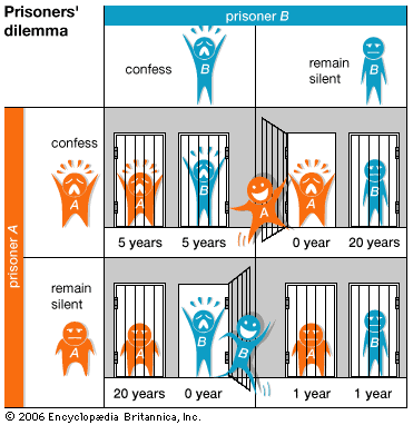
Prisoners’ dilemma: The moral of the story in terms of decisions in a legal setting: You have the right to stay silent and please shut the f* up and let your attoney to do the talk.

More examples can be found in this post.

Decision theory is similar to the game theory. The main differences are :

1. In the statistical context, the players are the statistician and “Nature”, who knows the true value of the parameter. In two-player game, both are trying simultaneously to maximize their winnings, whereas in decision theory nature chooses a state without this view in mind.

2. All statistical games allow statistician to gain information by sampling. However, it is the exploitation of the structure which such gathering of information gives to a game that distinguishes decision theory from game theory proper.

A real life example:

Medical diagnosis: Sometimes you never know until you open up the patient to see if the cancer is absent because of the limitations on imaging diagnosis. A surgeon needs to decide if a surgery (an action/ a decision) is necessary based on if the patient has cancer or not. There are 4 combinations between the 2 decisions and 2 conditions, thus 4 outcomes scored by %.

Combination 1: The presence of cancer is confirmed and the surgeon decides to perform a surgery. The score is 100% because that’s the best decision.

Combination 2: There is presence of cancer and the surgoen decides not to perform a surgery. The score is 0% because that’s the worst consequence.

Combination 3: Cancer is absent and the surgeon decides to perform a surgery. The score is 40% because it doesn’t results in serious consequence.

Combination 4: Cancer is absent and surgoen decides not to perform a surgery. The score is 85% because it’s a good decision and no consequence as well.

Models, Decision rules and Risk

Statistical model (class or family of distributions): The parameter \(\theta\) and data \(X\) are related through a model in which the distribution of \(X\) is determined by \(\theta\) The distribution when the parameter \(\theta\) is denoted \(P_\theta\) and we write \(X \sim P_\theta\). Formally, a model is written as the set of distributions for \(X\), \(\mathscr{P} = {P_\theta: \theta \in \Theta}\).

Decision rules: a non-randomized decision rule is a function \(\delta : \mathscr{X} -> \mathscr{D}\)

• The set of decision rules: \(\mathscr{D} => d \in \mathscr{D}, \theta \in \mathscr{D}\) and \(\delta(x) \in \mathscr{D}\) \(d=\delta(x)\)

• \(\delta\) prescribes a course of action for every observable dataset \(x\in \mathscr{X}\)

Risk: to evaluate a decision rule, we use risk \(R(\theta, \delta)\). It is the average loss \(L(\theta,d)\) between the estimand \(\theta\) and the estimator \(d\) –> an expected loss \(E_\theta\{ L[\theta,\delta(X)] \}\). One wants the estmator \(\delta(x)\) to be accurate, but just what measure of accuracy should be used is fairly arbitrary. Mean squared error (MSE) is the most famous measure. In 1820s, Gauss proposed the square of the error as a measure of loss. He defends his choice by an appeal to mathmematical simplicity and convenience.

Reference:

1. Mathematical Statistics: A Decision Theoretic Approach by Thomas S. Ferguson, Academic Press; 1st edition

2. Theoretical Statistics: Topics for a Core Course by Robert W. Keener, Springer; 2010 edition

3. Theory of Point Estimation by Erich L. Lehmann, George Casella, Springer; 2nd edition